1. INTRODUCTION
In recent years, wood demand has continued to increase across a number of sectors, such as construction, housing, and urban industries, thereby reinforcing the importance of a stable log supply and effective resource management. Moreover, wood products serve as significant carbon storage solutions, contributing to climate change mitigation efforts through long-term carbon sequestration in the built environment (Chang et al., 2018; Han and Lee, 2021; Han et al., 2022). In particular, the Korean red pine (Pinus densiflora) and Japanese larch (Larix kaempferi), which are widely used in Korea, are considered key species for ensuring supply stability. They are extensively used for sawn timber, plywood, fiberboard, and other wood products (Korea Forest Service, 2011–2024). However, uncertainties arising from climate change, logging policies, fluctuations in market demand, and the international timber trade have created challenges for long-term forest resource management (Kwon et al., 2015). Therefore, forecasting the future supply of major species is essential not only for efficient forest resource management, but also for establishing national wood supply policies (Lee and Kim, 2015; Lee et al., 2014).
Time-series models can serve as effective tools for projecting long-term trends in forest resources. Among these, the autoregressive integrated moving average (ARIMA) model has been widely applied to forecasting both short- and long-term values, and has demonstrated strong reliability and explanatory power (Bindel and Seifert, 2025). Based on historical observations, the ARIMA model estimates future supply patterns, making it a suitable method for analyzing timber supply under complex and uncertain conditions (Guo, 2024).
Jinman et al. (1996) applied an ARIMA(2,2,0) model to forecast the growth characteristics of Larix olgensis, including growth rate, ring width, and timber yield, and demonstrated that the ARIMA model explained the variation more effectively than a simple linear regression model (y = a + bx). Upadhyay (2013) employed ARIMA models to forecast India’s wood-based panel trade, selecting ARIMA(0,1,0) for exports and ARIMA(0,1,1) for imports based on the Bayesian information criterion (BIC), mean absolute percentage error (MAPE), and coefficient of determination (R-squared). The results projected that by 2020, exports and imports would reach approximately 2,892 and 2,422 million INR, respectively, representing increases of 170% and 127%, respectively, compared with 2011–12. Similarly, Thiyaharajan et al. (2025) used ARIMA(2,2,1) and ARIMA(2,1,1) models to predict India’s wood product trade up to 2027, estimating that exports would reach 27.7 million CUM RWE and that imports would reach 60.7 million CUM RWE.
Recent applications have expanded to include more sophisticated modeling frameworks. Banaś and Utnik-Banaś (2021) applied Seasonal ARIMA (SARIMA) and SARIMAX models to Polish timber price forecasting, achieving significant predictive accuracy at 95% confidence levels. In Indonesian researchers utilized ARIMA (1,2,0) and ARIMA(0,2,1) models to forecast national timber production across multiple product categories, projecting 10-year production volumes of 57.2 million m2 for roundwood, 24.8 million m2 for sawnwood, and 5.2 million m2 for plywood, based on Central Statistics Agency data from 2000–2009 (Huda et al., 2023). These studies highlight the applicability of ARIMA models in forecasting timber growth characteristics and international trade flows. However, research focusing on the domestic log purchase of major species, such as Korean red pine and Japanese larch, remains limited, particularly regarding time-series forecasting based on empirical data (Kim, 2013; Lee and Kim, 2015). These international applications demonstrate the widespread adoption of ARIMA methodologies across diverse forest sectors and geographic contexts. However, most international studies focus on aggregate timber markets, price forecasting, or export-import dynamics rather than species-specific domestic procurement patterns. This gap highlights the originality of applying ARIMA models to Korean species-specific log purchase forecasting, as domestic demand patterns for individual species require different analytical approaches compared to broad market trend analysis. Moreover, this species-specific approach holds particular significance in the context of Korea’s 6th Forest Master Plan, which emphasizes strengthening stable supply chains for domestic timber utilization in the carbon neutrality era (Korea Forest Service, 2018).
Accordingly, this study constructed ARIMA models based on the historical log purchase of Korean red pine and Japanese larch and forecasted their supply up to 2030. The results provide insights into the mid-term trends of these two species, highlighting the policy implications for uncertain management and stable resource supply. These findings are expected to provide valuable baseline data for future forest resource management and supply planning.
2. MATERIALS and METHODS
This study used the Market Survey of Timber Products, published annually by the Korea Forest Service, as the primary data source. The survey reports the annual log purchase (m3) of domestic timber industries registered for producing sawn timber, plywood, fiberboard, particleboard, and other wood products. Among these, the annual log purchase of Korean red pine and Japanese larch were used as key data for this study (Korea Forest Service, 2011–2024). Detailed yearly statistics of domestic log purchase from 2010 to 2023 are presented in Tables 1 (Korean red pine) and 2 (Japanese larch).
Data from Korea Forest Service (2011–2024).
Data from Korea Forest Service (2011–2024).
Log purchase was selected as the analytical basis for two reasons. First, in the Market Survey of Timber Products, it is the only indicator systematically reported at the species level (e.g., Korean red pine, Japanese larch), whereas other figures such as usage or input volume are aggregated by broader categories (e.g., coniferous or broad-leaved species). Second, log purchase directly reflects the annual procurement behavior of industries, while usage or input volumes may be influenced by production efficiency or inventory changes. Therefore, log purchase provides a clearer representation of market demand and supply trends for domestic species and is the most appropriate measure for forecasting analysis.
To forecast long-term fluctuations in the log purchase of Korean red pine and Japanese larch, this study employed the ARIMA model, which is widely used for time-series forecasting because of its ability to account for structural and stochastic variations (Box et al., 2015; Gopu et al., 2023; Jing, 2022; Lewis, 1982). In particular, ARIMA(p, d, q) integrates the autoregressive (AR), differencing (I), and moving average (MA) processes to capture temporal dependence. The dataset in this study is annual in frequency and relatively short in length, showing gradual long-term changes rather than distinct seasonal or high-frequency fluctuations. Under these conditions, ARIMA provides more stability and interpretability than more complex alternatives such as SARIMA, ARIMAX, or hybrid models, which typically require longer or higher-frequency datasets to yield reliable results. Therefore, the ARIMA model was deemed the most appropriate choice for this study.
The ARIMA models were constructed following the general procedure shown in Fig. 1. First, the time series data were transformed into a stationary process, and unit root tests such as the Augmented Dickey–Fuller (ADF) test and the Kwiatkowski–Phillips–Schmidt–Shin (KPSS) test were performed. Subsequently, the autocorrelation function (ACF) and partial autocorrelation function (PACF) were examined along with the Ljung–Box Q test to identify the appropriate order of the AR and MA terms. After parameter estimation, multiple candidate models were evaluated using statistical indicators, including the stationary R-squared, R-squared, root mean square error (RMSE), MAPE, maximum absolute percentage error (MaxAPE), mean absolute error (MAE), maximum absolute error (MaxAE), and normalized BIC.
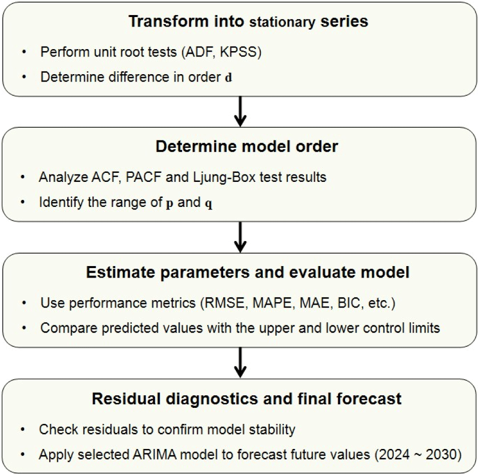
The interpretation and typical thresholds of these fit metrics are summarized in Table 3. This table provides a concise reference for evaluating model adequacy, where values close to 1 for stationary R-squared and R-squared indicate a good fit, while lower values of RMSE, MAE, MAPE, and BIC suggest higher predictive accuracy and parsimony.
Finally, the forecast intervals were derived by calculating the upper and lower control limits to provide a measure of prediction uncertainty. Based on these steps, ARIMA models were used to generate log purchase forecasts for the period of 2024–2030.
The ADF and KPSS tests were employed for unit root testing. Model identification and diagnostics were conducted using the autocorrelation functions ACF and PACF, as well as the Ljung–Box Q test. For the model estimation and forecasting of log purchase, the ARIMA procedure was implemented using SPSS (IBM SPSS Statistics, version 29.0.1.0, 171, IBM, Armonk, NY, USA). The outputs were analyzed and interpreted.
3. RESULTS and DISCUSSION
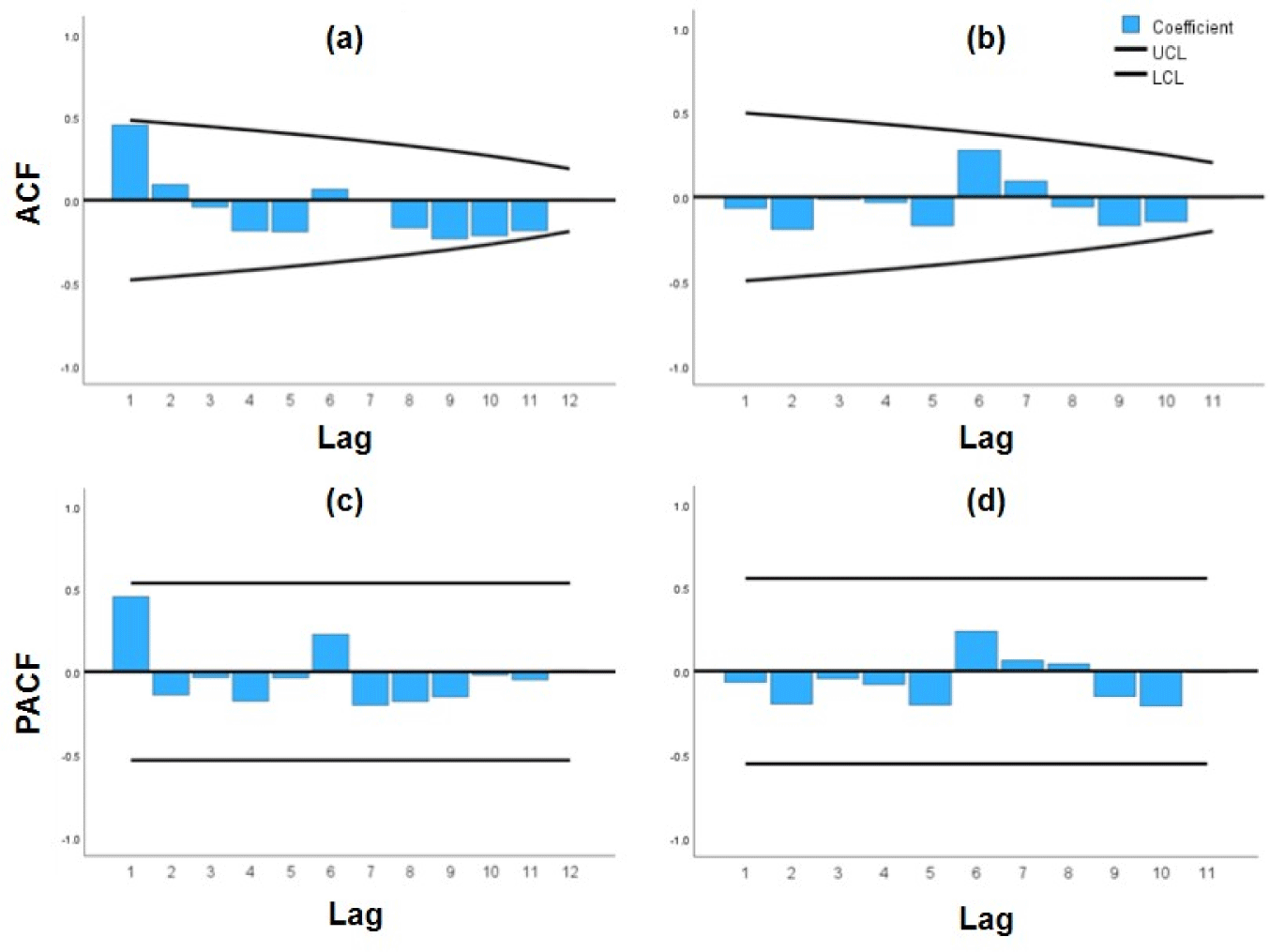
The annual log purchase of Korean red pine and Japanese larch, as presented in Tables 1 and 2, exhibited distinct long-term patterns. For Korean red pine, the volume generally increased from 2010 to 2021, peaking at 774,770 m3, but showed a declining trend in recent years. In contrast, Japanese larch displayed greater fluctuations, with an upward trend until 2015, followed by instability and a noticeable decrease after 2020. These results indicate that Korean red pine exhibited a relatively stable pattern of growth followed by decline, whereas Japanese larch showed higher volatility with a clear downward trend in recent years. Such long-term fluctuations are typical of non-stationary time series in which the mean and variance change over time rather than remaining constant (Yoon and Ahn, 2013). To statistically verify this property and to transform the nonstationary series into a stationary series, unit root tests were conducted using the ADF and KPSS tests. Based on the test results, first differencing was applied to achieve stationarity, and these changes can be visually confirmed through ACF and PACF plots before and after differencing (Figs. 2 and 3).
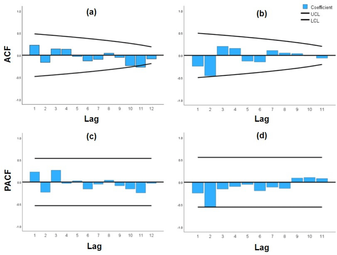
The test results are listed in Table 4. For the log purchase of Korean red pine without differencing, the ADF test showed a p-value greater than 0.05, indicating the presence of a unit root and the absence of stationarity. Similarly, the KPSS test produced a p-value of less than 0.05, suggesting nonstationarity. However, after applying the first differencing, the ADF test yielded a p-value below 0.05, rejecting the null hypothesis of a unit root, whereas the KPSS test produced a p-value greater than 0.05, confirming stationarity. Thus, the time series of Korean red pine log purchase achieved stationarity after the first differencing. In Fig. 2, some autocorrelation values in ACF exceeded confidence intervals before differencing, but all fell within confidence intervals after differencing, securing stability. However, residual autocorrelation remained relatively high at lag 2, indicating the need for additional stabilization by adjusting AR or MA orders during the model selection process.
| Wood species | Order of differencing | ADF p-value1) | KPSS p-value2) | Stationary result3) |
|---|---|---|---|---|
| Korean red pine | 0 | 0.98 | 0.1 < | No |
| 1 | 0.01 > | 0.1 < | Yes | |
| Japanese larch | 0 | 0.09 | 0.07 | No |
| 1 | 0.01 > | 0.1 < | Yes |
1) For Korean red pine, lag 4 was selected for the non-differenced data and lag 1 for the first-differenced data; for Japanese larch, lag 4 was selected for both.
A similar result was obtained for the Japanese larch. Without differencing, the ADF test produced a p-value greater than 0.05 and the KPSS test produced a p-value less than 0.05, both indicating non-stationarity. After the first differencing, the ADF test yielded a p-value below 0.05, and the KPSS test yielded a p-value above 0.05, confirming that the Japanese larch series also became stationary. In Fig. 3, ACF and PACF showed unstable autocorrelation structures, but became generally stabilized after differencing, with a slight spike observed at lag 6, suggesting the need for AR or MA model adjustments at orders of 6 or below.
This process reflects the standard procedure in time-series analysis, in which unit root tests and differencing are applied to ensure stationarity prior to ARIMA modeling (Box et al., 2015; Hyndman and Athanasopoulos, 2018). Numerous studies have employed this approach to verify the stationarity before conducting ARIMA-based forecasting (Atif, 2025; Rubio et al., 2023; Yoon and Ahn, 2013).
These results demonstrate that log purchase for both species achieved stationarity through first differencing, providing a reliable foundation for subsequent ARIMA model estimation.
After achieving stationarity through first differencing, orders p and q of the model were determined using the ACF, PACF, and Ljung–Box tests. In general, the ACF is useful for identifying the order q of the MA component, whereas the PACF is effective for determining the order p of the AR component (Bindel and Seifert, 2025; Hyndman and Athanasopoulos, 2018; Upadhyay, 2013).
As shown in Table 5, the results for Korean red pine log purchase indicated a significant negative autocorrelation at Lag 2 in the ACF (–0.46), and the PACF also showed a strong negative partial autocorrelation at the same lag (–0.546). Beyond this point, the correlations gradually decreased or were irregularly distributed, suggesting the appropriateness of considering the AR(2) or MA(2) models. The Ljung–Box test results confirmed that all lags had significance probabilities greater than 0.05, indicating that the residuals resemble white noise. Therefore, it was determined that ARIMA models for Korean red pine should be explored within the order of p, q ≤ 2.
Similarly, as shown in Table 6, the results for the Japanese larch indicated a weak positive autocorrelation at Lag 6 in the ACF (0.278), while the PACF also revealed a notable positive partial autocorrelation at Lag 6 (0.239). The Ljung–Box test results showed significance probabilities greater than 0.05 for all lags, indicating that the residuals were white noise. Accordingly, the ARIMA models for Japanese larch were considered appropriate within the order of p, q ≤ 6.
Abdulla and Hossain (2015) also stabilize the variance and achieve stationarity by applying a second differencing. Their results showed a significant spike at Lag 1 in both the PACF and ACF, suggesting that an AR(1) or MA(1) model would be effective for forecasting the yield, and they determined the model order accordingly. Similarly, Howard (2016) observed that the ACF gradually decayed after Lag 2, whereas the PACF sharply decreased, which corresponds to the growth process of the Gross National Product. Based on these findings, the AR(2) model is suggested to be suitable.
Based on the identified ranges of p and q, several ARIMA models were constructed, and their parameters were estimated. The model performance was assessed using the following multiple criteria: BIC, where lower values indicate higher generalizability; RMSE and MAE, which measure absolute errors; MAPE, which evaluates relative error levels; and MaxAPE and MaxAE, which assess extreme prediction errors. As presented in the Appendix, an extensive exploration of alternative models was conducted. Specifically, four alternative models were evaluated for Korean red pine, while thirty-five alternative models were examined for Japanese larch. From these candidates, two models were ultimately selected for each species based on balanced predictive accuracy and explanatory power. In addition, the explanatory power of the model was examined using the coefficient of determination (R-squared). The predictive reliability was further evaluated by comparing the upper and lower confidence limits of the 2030 forecasts, with narrower intervals indicating a more stable model.
As shown in Table 7, Korean red pine log purchase were best represented by the ARIMA(2,1,1) and ARIMA (2,1,2) models. For Japanese larch, ARIMA(1,1,5) and ARIMA(6,1,1) were identified as the most appropriate candidates.
ARIMA: autoregressive integrated moving average, RMSE: root mean square error, MAPE: mean absolute percentage error, MaxAPE: maximum absolute percentage error, MAE: mean absolute error, MaxAE: maximum absolute error, BIC: Bayesian information criterion, UCL: upper control limit; LCL: lower control limit.
For Korean red pine log purchase, both candidate models showed similar explanatory power (R-squared ≈ 0.43–0.44). However, ARIMA(2,1,1) achieved a lower RMSE (99,892 vs. 105,908) and MAE (72,359 vs. 72,799), as well as a smaller BIC value (23.81 vs. 24.13) compared to ARIMA(2,1,2), indicating a better overall performance. Additionally, a narrower confidence interval suggests greater forecasting stability.
For the Japanese larch, the ARIMA(6,1,1) showed slightly higher explanatory power (R2 = 0.404), its forecast interval was excessively wide, even yielding a negative lower confidence limit for 2030 (–21,079 m3), which undermines its practical validity. In contrast, ARIMA(1,1,5) demonstrated lower RMSE and BIC values, together with more reasonable confidence bounds, indicating that it provides a more stable and reliable forecasting performance.
Accordingly, ARIMA(2,1,1) was selected as the optimal model for Korean red pine, whereas ARIMA(1,1,5) was chosen for Japanese larch. This process follows the evaluation framework outlined by Bindel and Seifert (2025), which emphasizes the use of the stationary R-squared, R-squared, RMSE, MAE, MAPE, MaxAPE, MaxAE, normalized BIC, and forecast confidence intervals (upper and lower control limits) as key indicators for model selection.
Fig. 4 shows the residual ACF and PACF of the final ARIMA models for the Korean red pine and Japanese larch. Subfigures (a) and (b) show the residual ACF and PACF of the ARIMA(2,1,1) model for Korean red pine, whereas (c) and (d) present the results for the ARIMA (1,1,5) model for Japanese larch.
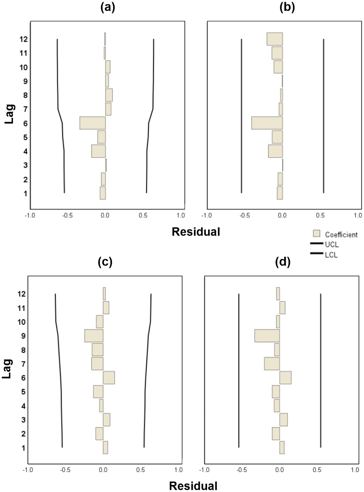
For the Korean red pine, both residual autocorrelations and partial autocorrelations were within the significance bounds, and no distinct patterns were observed. This indicated that the model successfully captured the autocorrelation structure of the data, leaving only white noise in the residuals.
For the Japanese larch, the residuals of the ARIMA (1,1,5) model also showed no significant autocorrelation in either the ACF or PACF, and the residuals were randomly distributed. This indicated that the model adequately captured the main time-series characteristics with no remaining systematic structure, confirming that the residuals resemble white noise.
Therefore, the selected models for both species were validated not only by goodness-of-fit measures, but also by residual diagnostics, ensuring their adequacy for forecasting and providing a reliable basis for prediction.
Fig. 5 shows the actual and forecasted log of Korean red pine and Japanese larch. Subfigures (a) and (b) present the ARIMA model forecasts from 2023 to 2030, along with the 95% confidence intervals (upper and lower control limits).
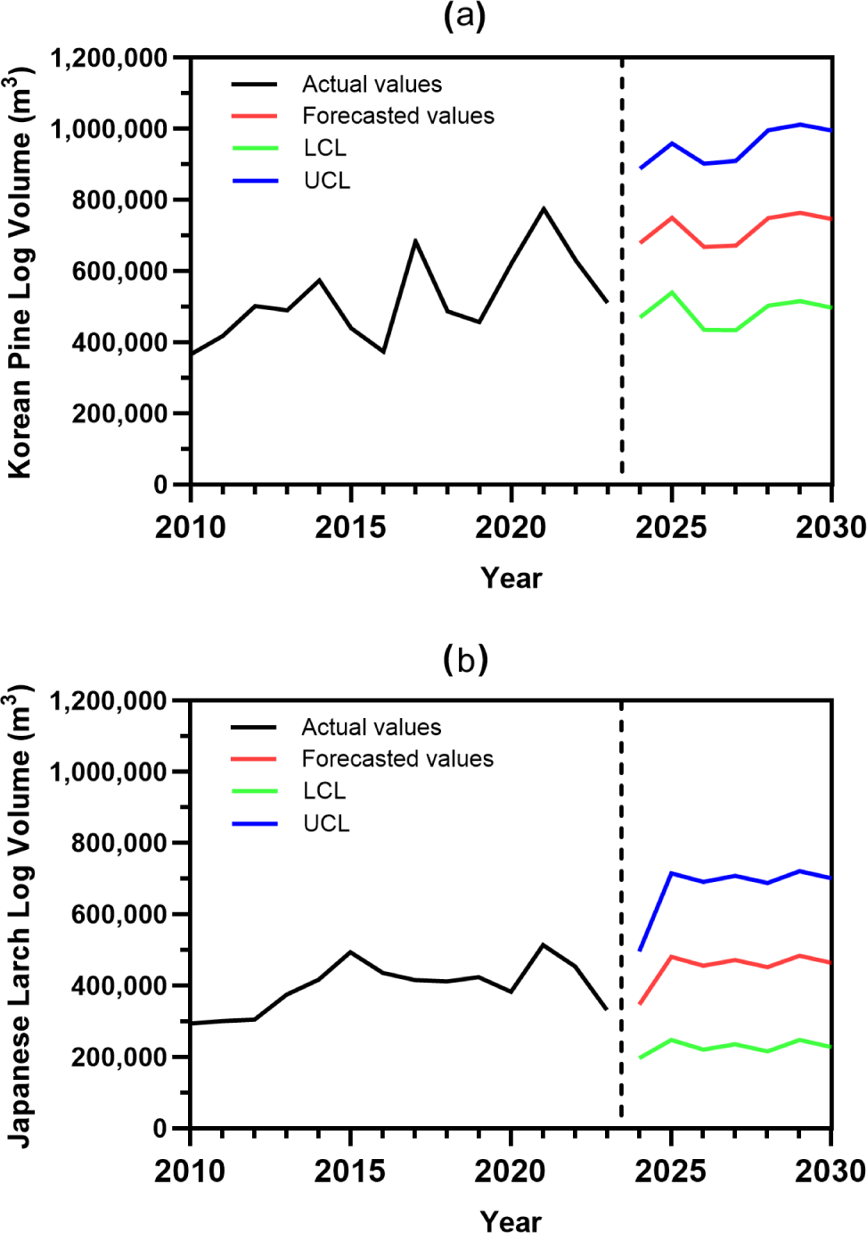
According to the forecast results, the log purchase of Korean red pine in 2030 was projected to be approximately 745,000 m3, with a confidence interval ranging from 497,000 to 995,000 m3. Although the absolute interval width was as large as 498,000 m3, the relative variability was only about 33%, suggesting a relatively stable log purchase outlook. In contrast, the Japanese larch was forecasted to be approximately 464,000 m3 in 2030, with a wider confidence interval of 227,000 to 700,000 m3. This interval width of 473,000 m3 corresponded to a relative variability of about 51%, indicating greater uncertainty in log purchase stability compared to Korean red pine.
These results suggested that Korean red pine is likely to maintain a relatively stable log purchase base, whereas Japanese larch exhibits greater variability and uncertainty. The wider prediction interval for Japanese larch highlights its vulnerability to market and environmental fluctuations, and indicates that forecasts should be interpreted as reflecting uncertainty rather than exact quantities. From a policy perspective, this implies the necessity of adaptive management strategies, including the diversification of supply sources, development of substitute species, establishment of contingency plans, and securing of long-term contracts. Recent studies have reported ongoing efforts to develop hybrid species and engineered wood products as potential substitutes for Japanese larch, reflecting the practical application of such adaptive strategies in Korea (Byeon et al., 2017; Choi et al., 2021; Galih et al., 2020; Gong et al., 2021; Ha et al., 2023; Kim et al., 2024; Yang et al., 2021). Such measures would help mitigate risks associated with the unstable outlook of Japanese larch.
The forecasts presented in this study can serve not only as simple statistical projections, but also as baseline information for resource management strategies that account for species-specific characteristics.
4. CONCLUSIONS
This study analyzed the time series of log purchase for Korean red pine and Japanese larch, and forecasted their log purchase from 2024 to 2030. The results indicated that the Korean red pine purchase is expected to remain at approximately 745,000 m3, with a relative variability of about 33%, suggesting a comparatively stable log purchase outlook. In contrast, the Japanese larch purchase is projected to be approximately 464,000 m3 in 2030, with a relative variability of about 51%, indicating higher uncertainty in log purchase stability. These findings imply that while the Korean red pine is likely to maintain a relatively stable log purchase base, while the Japanese larch requires complementary strategies, such as securing alternative species and strengthening resource management policies. Therefore, the results provide useful baseline information to support sustainable resource management and policy planning.
In regards to study limits, this study relied solely on historical log purchase data, and did not incorporate external factors, such as climate change, harvesting policies, or trade variables, which may influence future supply. Future research will aim to extend the dataset with longer time series and incorporate external explanatory variables, such as policy changes, climate variability, and economic indicators. By doing so, subsequent studies will be able to reduce uncertainty in long-term projections and provide more robust insights for policy and resource management.


