Development of a Computer Numerical Control (CNC)-Integrated Passive Autofocus for Continuous Wood Specimen Imaging Using Frequency-Domain Analysis

1. INTRODUCTION

Accurate wood-species identification is essential for industrial utilization, illegal-logging enforcement, and fundamental anatomical research. Traditionally, wood anatomists perform visual microscopic examinations to distinguish between species; however, the diversity and subtle anatomical differences among timbers mean that years of experience are required for reliable identification (Ravindran et al., 2020). This challenge has been faced in recent anatomical studies; for instance, delineation of juvenile and mature wood zones in Diospyros kaki requires precise cell-level imaging, underscoring the role of a stable focus in anatomical assessments (Kartikawati et al., 2024).

Illegal logging, which is estimated to generate 52–157 billion USD annually, drives deforestation and biodiversity loss worldwide (Silva et al., 2022). In addition, the enforcement of regulations, such as CITES, depends on rapid and trustworthy species recognition (Hwang and Sugiyama, 2021). Automated wood identification, which combines high-throughput microscopy, reliable autofocus, and explainable image analysis, is a critical tool in both conservation and commerce. Beyond identification, a consistent focus is required in wood utilization studies, such as the evaluation of teak sapwood for activated carbon production, where precise imaging is essential for interpreting anatomical features (Sutapa et al., 2024).

Deep learning-based approaches have demonstrated promising results in species classification using microscopic wood images (Kwon et al., 2017). For example, a convolutional neural network (CNN) model automatically identified Korean softwood species from transverse section images, achieving competitive accuracy without manual feature extraction. Building on this, ensembles of CNNs were introduced to further improve classification performance (Kwon et al., 2019), which highlighted the importance of large, high-quality image datasets and consistent imaging conditions for robust inference. More recently, the Mask R-CNN has been applied to the instance segmentation of softwood rays, which demonstrated reliable detection and measurement performance with microscopic wood images (Yoo et al., 2022).

These findings underscore that advances in imaging hardware-particularly autofocus-enabled, computer numerical control (CNC) integrated microscopy systems can directly contribute to enhancing AI-driven wood identification by supplying more consistent and sharper images for model training and employment.

Moreover, scanning electron microscopy-based analyses of adhesive bond-line performance have shown that even subtle losses in image clarity can compromise the interpretation of structural behavior (Kim et al., 2024), and complementary reviews of water vapor diffusion in adhesive layers have emphasized that reliable evaluation of bond-line durability depends on consistent microstructural observations (Zinad and Csiha, 2024).

In South Korea, where timber imports are subject to legal proof under recent regulations (e.g., the 2018 Act on the Sustainable Use of Timbers requiring proof of legal origin; Zeitlin and Overdevest, 2021), there remains a shortage of domestic anatomists, microscopy infrastructure, and reference databases, leaving inspection points without the tools needed to verify species instantly. Recent efforts to establish standardized property databases for Korean red pine have further highlighted the critical need for consistent imaging inputs to support reliable reference infrastructures (Park et al., 2024), and the inherently uneven surfaces of wood specimens cause any preset focus to drift as the stage moves to a new area, requiring continuous refocusing to maintain image quality. Such unevenness is a major issue in drying processes, where internal water transport strongly influences defects, and recent work on large-cross-section red pine timber has demonstrated that pretreatment can mitigate these problems (Batjargal et al., 2023).

Moreover, reliable image-based analyses are essential not only for species recognition and sustainability (Hadi et al., 2022) but also for broader material characterization. Studies on clonal teak trees have demonstrated that ImageJ-based anatomical measurements of growth and density rely heavily on image clarity to ensure reproducibility (Nugroho et al., 2024).

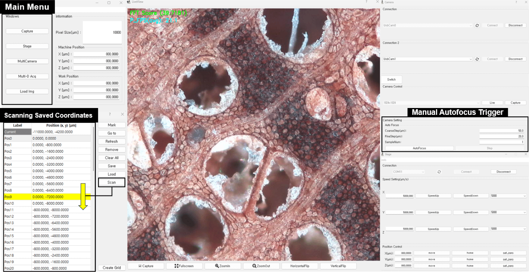
To address this problem, our objective was to develop a low-cost, CNC-integrated autofocus module that enables rapid, repeatable focus adjustment across large wood-specimen surfaces. The entire autofocus module was designed for modular CNC integration such that it could be retrofitted to existing microscope stages. The stage executes a simple “move, stop, autofocus, capture, move” loop under standard G-code control, capturing each coordinate only once the focus has been optimized. This modularity allows large-area tiling with guaranteed focus consistency and eliminates the need for manual refocusing between positions, dramatically increasing throughput in automated wood-imaging workflows.

Autofocus methods can be broadly classified into active and passive approaches (Chen et al., 2010; Peddigari et al., 2005). Active autofocus employs auxiliary optical devices, such as infrared or ultrasonic sensors, to calculate the distance to the specimen surface, providing rapid focus adjustment but requiring additional hardware that increases the system cost.

In contrast, passive autofocus relies solely on image-derived metrics and can be implemented in either the spatial or frequency domains. Spatial-domain techniques evaluate focus quality through measures such as the image Laplacian, which computes the second derivative of the pixel intensity to quantify edge sharpness, and the Sobel operator, which estimates first-order intensity gradients, as well as various statistical methods (Wu et al., 2022).

Frequency-domain methods, on the other hand, apply the fast Fourier transform (FFT) to convert image data into its spectral components. Signal and noise occupy different frequency bands, therefore these methods generally exhibit superior anti-noise performance compared to spatial-domain metrics (Li et al., 2024). By adapting passive autofocus strategies, our CNC-regulated module can maintain optimal focus across micrometre-scale height variations in wood specimens, yielding consistently sharp microscopic images, even on inherently uneven surfaces.

2. MATERIALS and METHODS

2.2. Methods

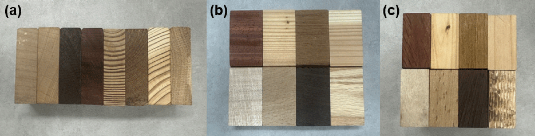
The wood samples were examined using three principal planes: the transverse [Fig. 1(a)], longitudinal [radial; Fig. 1(b)], and longitudinal planes [Fig. 1(c)]. As illustrated in Fig. 1(a), the transverse plane clearly reveals both the growth-ring anatomy and the boundaries between the heartwood, sapwood, earlywood, and latewood (Arisandi et al., 2023). All microscopic imaging was performed on cross-sections of the wood, because in preliminary trials, we found that using perfectly flat surfaces made observations of the cross-section far easier than using radial or tangential faces, maximizing image clarity and reproducibility.

Fig. 1. Photographic overview of the eight wood block specimens used in this study. (a) Transverse, (b) longitudinal (radial), and (c) longitudinal surfaces.

Download Original Figure

The GRBL-controlled board drives three stepper-motor axes. The X- and Y-axes translate the workable beneath the z-axis gantry, which carries two aligned cameras. The wood specimens were arranged on the Y-stage and positioned incrementally for imaging purposes.

Each 70 mm 20 mm sample was scanned along blue lines from its starting position (red triangle) to its halt position (green squares; Fig. 2). No automatic boundary-recognition procedure was used to define the scan path. Instead, all X-Y target coordinates were specified manually prior to acquisition (via the control GUI), and the specimen positioning was manually adjusted when needed. To control the spacing between consecutively scanned regions and support downstream stitching in future studies, we intentionally introduced an overlap between adjacent tiles. During capturing, subsequent coordinates were offset by 800 μm along either the X or the Y axis; this fixed step size yielded a small but consistent overlap at the tile boundaries and prevented gaps.

Fig. 2. CNC based wood-surface scanning system and schematic of the wood scan path. CNC: computer numerical control.

Download Original Figure

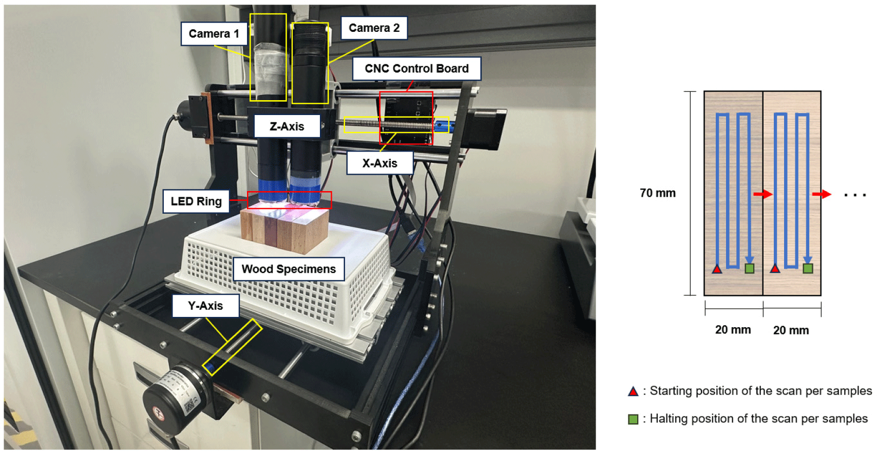
Upon completion of the scanning process for one sample, the head shifted along the X-axis by 20 mm, and the next sample was scanned using the same process, yielding continuous scan coverage of the defined surface to be observed.

To enable real-time blur detection on wood specimen surfaces, we implemented a GPU-accelerated sharpness metric based on FFT and a two-stage hill-climbing algorithm using Python. All processing was performed on 1,024 × 1,024-pixel frames using NVIDIA GPUs and the CuPy Library (https://github.com/cupy/cupy).

In practice, although we applied FFT due to its efficiency, the underlying mathematical operation used was discrete Fourier transform (DFT). The DFT of an M × X image I (x, y) is defined as

$$F\left(k,l\right)={\displaystyle \sum _{x=0}^{M-1}{\displaystyle \sum _{y=0}^{N-1}I\left(x,y\right)}{e}^{-j2\pi \left(\frac{kx}{M}+\frac{ly}{N}\right)}}$$

(1)

Where I (x, y) is the intensity of the input image at pixel I (x, y), M and N are the width and height of the image (in pixels), K and I are the horizontal and vertical frequency indices, respectively; and $j=\sqrt{-1}$ is the imaginary unit. The direct computation costs O (M²N²) operations are prohibitively high for a 1,024 × 1,024 frame. In practice, we used the FFT O ((MN) log(MN)) algorithm that produces identical results (Changela et al., 2020).

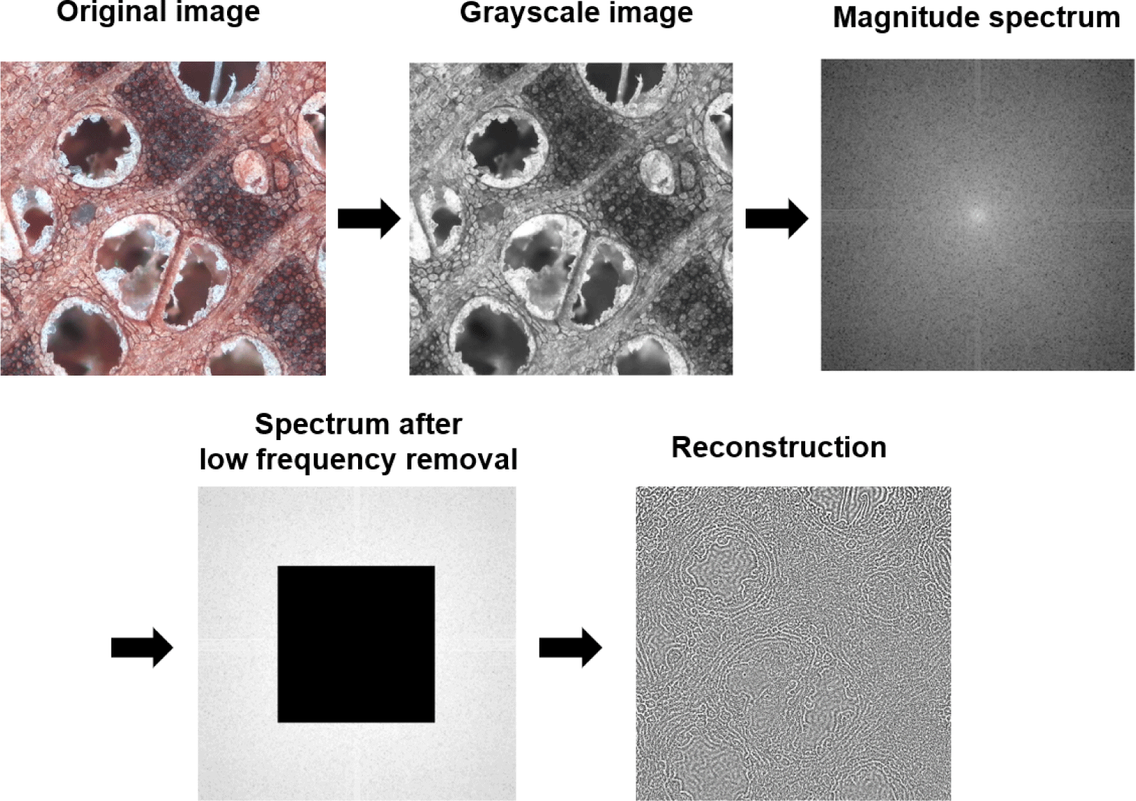
Before applying FFT, we converted any incoming color frame into a single-channel grayscale image, as shown in Fig. 3. This collapsed the RGB channels into luminance, ensuring that the FFT only measured intensity variations (edges and textures) without being skewed by color content, and provided a reduced-complexity representation that eases the computational load and accelerates processing (Lin et al., 2024).

Fig. 3. End to end fast Fourier transform-based blur-emphasis pipeline.

Download Original Figure

The inverse transform is calculated as follows:

$$I^{\prime }\left(x,y\right)=\frac{1}{MN}{\displaystyle \sum _{x=0}^{M-1}{\displaystyle \sum _{y=0}^{N-1}{F}^{\prime }\left(k,l\right)}{e}^{j2\pi \left(\frac{kx}{M}+\frac{ly}{N}\right)}}$$

(2)

On the GPU, each frame was streamed to the device via memcpyAsync on a non-blocking CUDA stream. Then, we performed the following sequence of spectral operations to suppress blurring and emphasize the edges:

1. Computed the real-input 2D FFT.

2. The zero-frequency component was moved to the center of the spectrum, where it appeared as the brightest point in the magnitude image, which represented the image’s overall mean intensity, while the intensities fell radially, indicating higher spatial frequencies as it moves outward.

3. Central low-frequency removal to zero out a square block of coefficients, such that subsequent processing only operated on detail-rich frequencies.

4. Undid the earlier shift, restoring the spectrum’s natural indexing.

5. The spatial image Î (x, y) was reconstructed from the masked spectrum. All very low frequencies are eliminated, therefore the resulting image highlights the edges and fine texture, which is an essential prerequisite for a reliable blur metric.

The zero-frequency component moving process in Step 2 is not mathematically required for the FFT itself, but it significantly improves both visualization and processing convenience. In the raw FFT output, the zero-frequency component is located at the array corners, with the low-frequency information split across the four quadrants. By shifting the zero-frequency component to the center, the spectrum becomes radially symmetrical, with low frequencies concentrated at the center and high frequencies radiating outward. This layout is easier to interpret by humans and allows for simple isotropic masking operations, such as removing a central block of coefficients without having to treat multiple disjoint regions at the array corners.

Next, we compute the focus score S by applying decibel-style compression to the reconstructed amplitude |Î (x, y)| and averaging over all pixels:

$$S=\frac{1}{MN}{\displaystyle \sum _{x=0}^{M-1}{\displaystyle \sum _{y=0}^{N-1}20{\log }_{10}}\left(\left|\widehat{I}\left(x,y\right)\right|+\epsilon \right)}$$

(3)

Where ε prevents logarithmic singularities. The 20log₁₀ form to express the amplitude compresses the wide dynamic range of the FFT and sensitively reflects even small high-frequency losses, ensuring that blurry frames yield significantly lower scores (Fig. 4).

Fig. 4. Saved focus score thresholds over time. The graph on the left is a full sweep of the saved threshold values, showing a clear peak and symmetrical drop-off. The graph on the right side is a zoomed in view of the saved values below 0 db, where the focus-score algorithm’s natural jitter dominates.

Download Original Figure

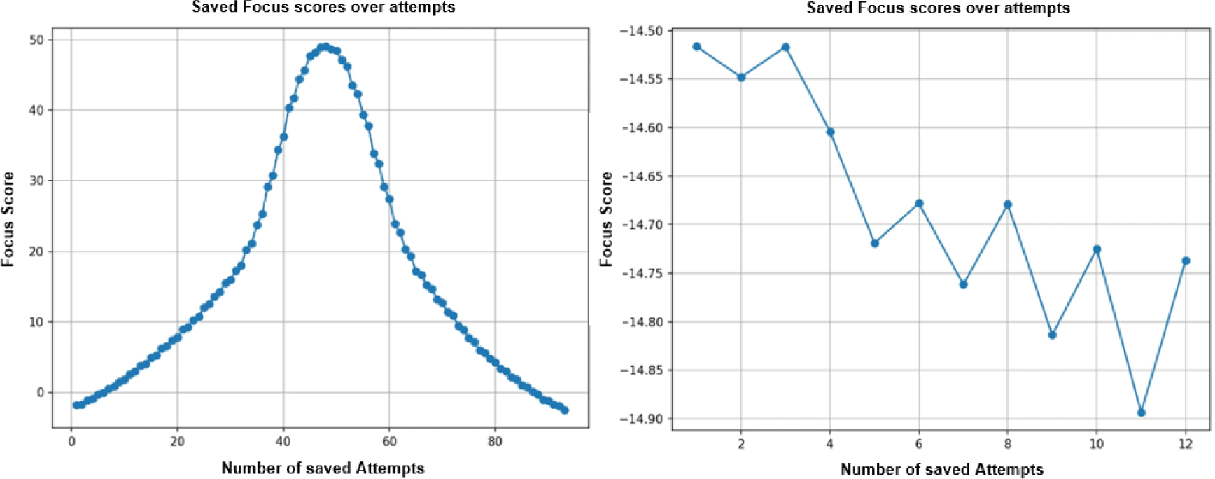
To locate the optimal focus position, we applied a two-stage hill-climbing search (Jia et al., 2022) along the Z-axis, as shown in Fig. 5. In the coarse search, the stage moves up or down from the initialized Z position in increments of ΔZ coarse, measuring S after each move. It continues in a direction that increases S and halts when no further improvement occurs (either owing to a score drop or exceeding the reversal limits). Then, the fine search repeats this procedure from the coarse result using smaller increases in ΔZ fine, precisely converging on the local maximum of S. The Z-axis step sizes for coarse and fine searches were chosen to match our stage’s 1.8° two-phase stepper motors, which move 10 μm per pulse, and to exceed the natural jitter of our FFT-based focus score. The 10 μm resolution was derived directly from our CNC motor’s full step angle attached with a 2 mm lead screw and using the following calculation:

Fig. 5. The four steps of autofocus after the initialization process. 1) Coarse forward scan locates an approximate focus maximum. 2) Reverse coarse scan refines the position from the opposite direction. 3) Fine forward scan around the coarse peak yields a high-precision focus estimate. 4) Reverse fine scan provides the final Z-axis position adjustment.

Download Original Figure

$$\Delta x=2mm\times \frac{{1.8}^{\circ }}{{360}^{\circ }}=0.01mm=10\text{μ}m$$

(4)

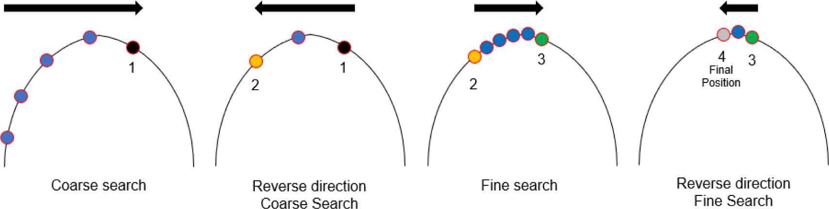
Although microstepping was used for smooth motor movement, it only smoothed the motor drive currents in the CNC board (Fig. 2) and did not alter the fundamental full-step size of the chosen stepper motor (Bednarski et al., 2021). Therefore, we set the fine-search increment to ΔZ = 10 μm to prevent consecutive measurements from overlapping within the ± 5 μm focus jitter window, and we selected ΔZ coarse = 50 μm to reliably bracket the true focus peak in the coarse stage, avoiding unintentional overshooting.

To avoid false starts in the low-score region, autofocus was initiated by loading the saved X and Y coordinates and oscillating the stage up and down until the focus score increased above zero, where our empirically determined boundary beyond which score fluctuations no longer overlapped, before commencing the two-stage hill-climbing routine.

The acceptable sharpness range around the true focal plane is called the lens’s depth of focus (DOF; Young et al., 1993). Once the Z-axis position fell anywhere within the DOF range, the image quality remained constant. This implies that the fine-search stage does not need to chase the absolute maximum focus score at every micrometer step, and converging into the lens’s DOF is sufficient to guarantee sharp images while minimizing unnecessary Z-axis control.

In this study, the DOF was defined by the following diffraction-based expression:

$$\Delta z=\frac{\text{λ}}{4\cdot n\cdot \left(1-\sqrt{1-{\left(NA/n\right)}^2}\right)}$$

(5)

Where λ denotes the wavelength of the (quasi-monochromatic) illumination, NA is the objective’s numerical aperture, and n represents the refractive index of the medium separating the lens form the specimen. This formulation originates from the diffraction theory, in which the axial range is determined by the point at which the accumulated phase deviation causes the Airy disk to surpass the permissible blur size in the image plane.

When the numerical aperture is moderate (NA ≪ n, the square-root term can be approximated by a first-order Taylor expansion:

$$\sqrt{1-{\left(NA/n\right)}^2}\approx 1-\frac{{\left(\frac{NA}{n}\right)}^2}{2}$$

(6)

Substituting this into Equation (5) yields:

$$\Delta z\approx \frac{\text{λ}}{2N{A}^2}$$

(7)

This simplified formula is used for quick estimations, because it avoids the nested square root and closely matches the exact form in the low- to mid-regime. The approximation is valid here because our microscope geometry fixed the distance between the image sensor and the internal optics of the camera. Under this fixed geometry, the DOF refers specifically to the allowable displacement of the image plane (in the sensor space) and should not be confused with the depth of field, which describes the object-space range and scales differently with magnification. The optical setup from the lens to the sensor is rigid, therefore the DOF value computed using Equation (5) (or its simplified form) directly corresponds to the z-axis tolerance in the CNC stage program (Fig. 6).

Fig. 6. Graphical user interface for automatic microscope image acquisition and stage control.

Download Original Figure

In our autofocus implementation, this DOF limit was used as a stop condition for fine-stage motion. Once the focus score predicts that the Z position is inside the calculated DOF, the hill-climbing search halts, ensuring efficient operation while maintaining image sharpness.

3. RESULTS and DISCUSSION

In this experiment, we evaluated the performance of our GPU-accelerated FFT-based sharpness metric for the identification of various wood specimens. Specifically, we tested whether our autofocus method could find precise Z-axis locations in various samples, and how fast this method could scan multiple specimens.

The Fig. 7 shows 12 sequential images per sample captured at 1,024 × 1,024 resolution using our 4 × / 0.13 phase-contrast objective lens and the USB camera module. In our five-sample run, the system acquired 200 images in approximately 18 min and 20 s. The CNC stage stepped the Y-axis 10 times (800 μm each) then shifted the X-axis and repeated the process, yielding 40 images per specimen.

Fig. 7. Examples of sequential autofocus scanning capture of various wood specimens over adjacent X–Y positions, demonstrating consistent focus despite variations in sample surface topography. All images were acquired using the Nikon Plan 4 × 0.13 phase objective, whose diffraction-limited depth of focus, from the simplified approximation △z ≈ λ / (2NA²) with λ ≈ 0.55 μm, is about △z ≈ 16.27 μm in the air. Representative microscopic snapshots of various wood species under the proposed FFT-based autofocus system of the Fagus grandifolia, Cryptomeria japonica, Pterocarpus soyauxii, Acer saccharum, Tectona grandis, Quercus spp. Millettia laurentii, and Larix kaempferi were shown, arranged in rows 1–8 in the order listed. FFT: fast Fourier transform.

Download Original Figure

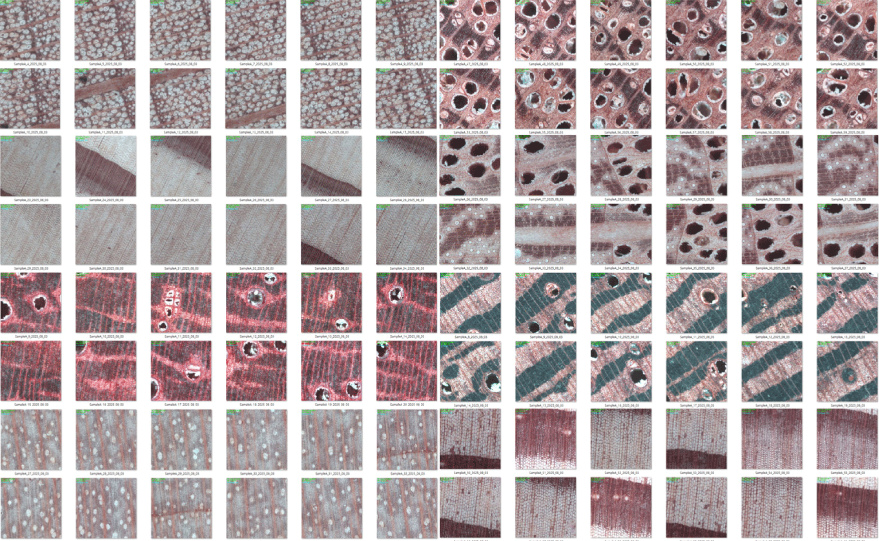
After initializing the prefocus sequence for each sample, each coordinate required an average of 6.61 seconds to achieve an optimal focus position. More critically, the autofocus accuracy never exceeded ± 10 μm deviation, which is well within the DOF, regardless of wood anatomy or surface unevenness. This repeatable performance confirmed that our FFT-based metric robustly locks onto true defocus rather than native high-frequency textures across a variety of sample types.

Each move triggered a GPU-accelerated FFT score calculation, forming a closed loop of stage motion, image capture, score computation, and direction decision in near-real time.

By overlapping the data transfer and kernel execution on CUDA streams and reusing the FFT plans, our GPU pipeline reduced the planning overhead by over 90%. Compared to CPU-only implementation, the end-to-end throughput was more than three times faster, achieving approximately 18 fps for combined focus detection.

Although the FFT excels in processing individual and static frames, our five-sample benchmark showed similar scan times on the CPU and GPU (18 min); the true strength of the GPU lies in continuous, real-time analysis. By grabbing each frame “on the fly,” feeding it directly into a reusable FFT plan, as a future work layering a lightweight wavelet transform for multi-scale feature extraction could be used while sustaining the number of frames per second. This provides an avenue for achieving true real-time focus without pausing the motor movement (Table 1).

4. CONCLUSIONS

In this study, the core of our system met the need for a robust sharpness measurement algorithm that can reliably distinguish true focus from spurious texture across the highly uneven and intricate surfaces of wood specimens. A key technical challenge addressed in this study was differentiating genuine defocus from native high-frequency features in the wood microstructure. By isolating the relevant frequency bands, our FFT-based sharpness metric successfully distinguishes true blur from structural texture. This selective sensitivity is essential to ensure a consistent focus with anatomically complex specimens. This capability underpins the ability of the system to generate uniformly sharp images across species, even for field deployment.

To keep pace with the scanning stage and avoid bottlenecks, all FFT computations, including plan generation, data transfer, and spectral masking, were fully offloaded to the GPU using pinned memory transfers, non-blocking CUDA streams, and plan caching. This pipeline achieved the throughput necessary for a continuous focus evaluation at 18 fps or higher.

To ensure that non-specialist operators could harness this technology in the field, we wrapped the autofocus routines within an intuitive graphical interface. With a clean layout for parameter tuning (motor control, threshold levels, and coarse/fine step sizes), and live visual indicators of the current focus score and stage position, users can configure, monitor, and troubleshoot the autofocus process without writing code or diving into low-level GPU settings.

In addition, to address the uneven image quality caused by frame-to-frame brightness variations during continuous capture, implementing an image-stitching pipeline–first aligning and merging overlapping frames, and then normalizing and correcting their brightness to generate a single, seamless, high-quality composite–could be considered in future work (Mohammadi et al., 2024).

Moreover, because our FFT-based sharpness metric operates purely in the frequency domain and cannot capture temporal information, we will investigate it using a discrete wavelet transform (DWT) in the future (Yang et al., 2025). By decomposing each frame into both time and frequency, DWT should allow us to identify and skip moments, for example, during motor-induced vibrations, when the image quality briefly degrades, and instead select and store only the fine-focused frames at each timestamp.

By meeting these requirements, the proposed autofocus technique lays the foundation for automated, large-scale wood imaging workflows, strengthening enforcement against illegal logging, and the generation of comprehensive anatomical datasets. Given its modular architecture and reliance on low-cost components, the proposed autofocus system can be readily retrofitted into existing laboratory- or field-grade wood-imaging setups, thereby providing an affordable pathway for high-throughput anatomical analysis. Beyond its technical contributions, such reliability in imaging can also support broader societal goals, as public surveys have shown that confidence in wood as an ecofriendly and health-promoting material strongly influences its cultural adoption (Han and Yang, 2022).

One limitation is that although GPUs are well-suited for streaming, our current pipeline still follows a sequential per-frame pattern (capture → host transfer → FFT scoring → idle), which prevents overlap between computation and data movement. In addition, repeated transfers between the CPU and the GPU introduce I/O bottlenecks. For future large-scale or real-time deployments, we plan to adopt a more GPU-friendly streaming design to minimize host-device traffic and enable true end-to-end concurrency.