
1. INTRODUCTION
Wood is the most dominant forest product for commercial use in various industries as raw material and to support the daily life of humans, such as building materials, furniture, craft arts, and many others. In identifying the wood, the visual inspection of various wood tissues is a common method (Hwang et al., 2020). Wood species are very diverse, but still have unique characteristics that can be distinguished from each other. Therefore, an accurate and reliable wood classification system based on the image classification method needs to be developed.
Several previous works related with microsopic analaysis of the wood surface can be mentioned as follows. Savero et al. (2020) investigate wood characteristics of 8-year-old superior teak from Muna Island by observing macroscopic and microscopic anatomical characteristics. This study showed differences in the characteristics of the higher wood portion, wood texture, growing ring width, and wood specific gravity which were categorized as a Strength Class of III (Savero et al., 2020). Furthermore, Jeon et al. (2020) researched the anatomical characteristics of Quercus mongolica which was attacked by oak wilt disease, the anatomical structure of infected wood, deadwood, and healthy wood. The results of the study that showed a big difference between wood affected by oak wilt and healthy wood was the tyloses ratio (Jeon et al., 2020). Finally, Jeon et al. (2018) conducted a study on the characteristics of Korean commercial bamboo species (Phyllostachys pubescens, Phyllostachys nigra, and Phyllostachys bambusoides). The research resulted in crystal properties, vascular bundle, fiber length, vessel diameter, and parenchyma, as well as the length and width of the radial and tangential sections (Jeon et al., 2018).
Salma et al. (2018) proposed a wood identification algorithm by combining Daubechies Wavelet (DW) and Local Binary Pattern (LBP) methods (Salma et al., 2018) as the pattern extractor. The pattern was then classified by using support vector machine (SVM) classifier. Sugiarto et al. (2017) developed a wood identification algorithm based on cooperation between the histogram of oriented gradient (HOG) and the SVM classifier (Sugiarto et al., 2017). Meanwhile, Kobayashi et al. (2019) developed a method for statistically extracting the anatomical features of Fagaceae (Kobayashi et al., 2019). This approach could help to reveal some new aspects of wood anatomy that might be difficult in conventional observation. The next reference is reported by Hadiwidjaja et al. (2019). The paper implemented the LBP and Hough transform methods to improve the extract of the wood feature.
Classification has become one of the main topics that has attached much attention in recent years. Many methods have been developed for classification purposes. Nowadays, the convolutional neural network (CNN) emerges as a powerful visual model with an outstanding performance in various visual recognition and classification problems, for instance, as presented in the papers of Yu et al. (2017), and Levi and Hassner (2015). Yu et al. (2017) developed an efficient CNN architecture to boost the hyperspectral image classification discriminative capability. Levi and Hassner (2015) proposed a simple convolutional net architecture that can be used even when the amount of learning data is limited. Their method was evaluated with the Adience benchmark for age and gender estimation and successfully outperformed other current methods. The Adience dataset is a dataset of face images acquired at common imaging conditions. Therefore, variations of object appearance, poses, and environmental light are found since the photos were taken in free situations. The CNN method can provide excellent classification results, but it still has a challenge in the number of data sets needed to make the classifier well trained (Yu et al., 2017; Levi and Hassner, 2015; Maggiori et al., 2016; Marmanis et al., 2015).
Several previous studies that became references in the use of CNN in the classification and identification process include works of Kwon et al. (2019), Kwon et al. (2017) and Yang et al. (2019). In the first paper, Kwon et al. (2019) used the ensemble model LeNet2, LeNet3, and MiniVGGNet4 to classified Korean softwood with the F1 score reaching 0.98. In the second paper, Kwon et al. (2017) developed an automatic wood species identification system utilising CNN models such as LeNet, MiniVGGNet, and their variants. The research showed a sufficiently fast and accurate result with 99.3% accuracy score by LeNet3 architecture for five Korean softwood species. In the last paper, Yang et al. (2019) used the ensemble methods of two different convolutional neural network models, i.e., LeNet3 and NIRNet. The ensemble methods were applied to lumber species with the average F1 score of 95.31%.
In this wood classification research, we attempted to identify the microscopic wood image. By following the successful example in the paper discussed earlier, the CNN method becomes one of the potential approaches to solve the microscopic wood image classification. In overcoming the small number of wood datasets to train the CNN classifier, as mentioned in several studies in the paragraph above, to get a good CNN classifier requires an adequate quantity of datasets in the training process. A sample selection process is proposed before the microscopic image of wood dataset enters the classification stage using the CNN method. Inside the sample selection process, the wood image is cropped into several sections at a specific size. We assumed that even though it only uses certain image segments, it has some characteristics that can distinguish one species from another, such as vessel size, the density of vessels, colour, and transverse wood fibre.
The remaining part is organised as follows. Section 2 presents the data sets used in the research, the sample selection process, the proposed CNN architectures, and the proposed classification algorithm. Section 3 furthermore presents all experimental results started from the sample selection, training, and testing results. The last section, Section 4, provides the conclusion and future work.
2. MATERIALS and METHODS
The wood species is commonly recognised by examining a small piece of wood as a sample. In this Japanese Fagaceae wood classification research, we observed the microscopic features of the wood. The commonly observed microscopic features are vessels, parenchyma, rays, and others (Schoch et al., 2004; Prislan et al., 2014). Observations are made by collecting micro cores and observing them under a light microscope (Prislan et al., 2014).
This research used a wood dataset obtained from the Research Institute of Sustainable Humanosphere (RISH), Kyoto University, Japan. The dataset consisted of microscopic images of nine species of Fagaceae woods. Table 1 presents the list of wood.


Each image in the dataset was stored as a TIFF file with the 4140 × 3096 - pixel dimension. The existing dataset was divided into three groups: training data, validation data, and test data. Data for test consisted of 27 images (3 images from each species), data for validation consisted of 18 images (2 images from each species), and data for train consisted of 120 images (as the rest of images).
The proposed method used a small segment of the image as an input. This procedure was defined by considering the size of the original image and limited dataset availability of 165 images. The image had a dimension of 4140 × 3096 pixels with a size of approximately 38 MB. The implementation of an image processing algorithm on an image with a large size could cost the computer resources and computational time. Moreover, as informed from the previous section, the minimum number of datasets can result in overfitting and low generalisation capabilities of the CNN model.
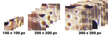
The process of taking specific segments of the input image consisted of 3 categories based on the sample area size. The first category was small that would crop the image with a size of 100 × 100 pixels and produced 1230 sample areas for each image. The second category was medium that would crop images with a size of 200 × 200 pixels and produced 300 sample areas for each image. Moreover, the last one was the large category to crop images with a size of 300 × 300 pixels and produced 130 sample areas for each image.
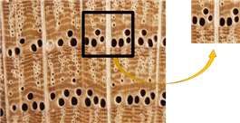
Fig. 1 depicts the more specific and detailed features provided by the selected area sample. The CNN model trained on specific and detailed features resulted in a CNN model that had excellent generational capabilities though with the limited dataset provided.
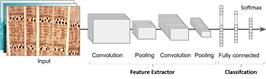
CNN is a neural network architecture used for prediction when the input observations are images, which is the case in a wide range of neural network applications (Seth, 2019). In principle, CNN mimics the visual cortex. It is based on studies as conducted by Neocognitrons in 1980 (Fukushima, 1980), which gradually evolved into what is now called as convolutional neural networks (Géron, 2019). CNN is very similar to ordinary neural networks and still consists of neurons with weights that can be learned from data. Each neuron receives several inputs and performs a dot product. In general, CNN has three main layers: the convolution layer, pooling layer, and fully connected layer (Sewak et al., 2018).
Fig. 2 shows that the typical CNN architecture piles up several convolutional layers (followed by activators), and pooling layer. Several convolutional layers (followed by activators), other pooling layers, and so on until the final layer produces several predictions (for instance, the softmax layer outputting several estimated class probabilities) (Géron, 2019).
In practice nowadays, very few people train entire convolutional networks from scratch. They do not choose this way for several reasons, such as many data required in the process to train the CNN model; lots of parameters (weights) to be trained and to avoid overfitting. The transfer learning is a solution for the problem. Five CNN architectures have been designed by applying transfer learning to fit in the sample selected data set.
Transfer learning is a machine learning technique that reuses the trained and developed models from one task into the second task. It refers to the situation whereby what has been learned in one setting is exploited to improve optimization in another setting (Hussain et al., 2019). Some examples of popular pre-trained models for transfer learning are VGG-16, MobileNet, ResNet-50, and DenseNet.
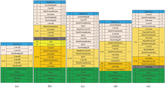
Fig. 3 illustrates the architecture of each model. Each base architecture was cut into a particular network depth, such as VGG16 (Simonyan and Zisserman, 2014) at the 19th layer, ResNet50 (He et al., 2016) at the 39th layer, MobileNet (Howard et al., 2017) at the 23rd layer, DenseNet121 (Huang et al., 2017) at the 51st layer, and Xception (Chollet, 2017) at the 42nd layer. All layers were cut after the specified layers. Furthermore, a new fully connected layer would be used to fit the nine species/class of wood. The use of shallow network depth aimed to prevent the network from losing the essential features of the wood. The deeper the network, the more detailed the features will be produced; and this can affect the sample selected image with the features that are sufficiently detailed to be lost.
Algorithm development consisted of two main steps. The training process initiated the step (Fig. 4) followed by the testing process (Fig. 5) as the second step.
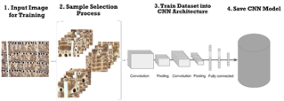
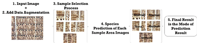
The training process began with a sample selection process, as described in subsection 2.2. Furthermore, each architecture as in subsection 2.3 was trained in each sample selection size category (small 100 × 100 pixels, medium 200 × 200 pixels, and large 300 × 300), therefore each architecture could produce 3 models, and in total for 5 architectures, there would be 15 models.
In the testing process, augmentation data would be added to the test sets. The addition of data augmentation aimed to add data variation and make the testing process able to describe a more general situation. The augmentation process was carried out by rotating the image, thereby increasing the total number of test data to 54 images. Furthermore, test sets entered the sample selection stage. However, the difference was that not all sample areas for each image was going to be used. The optimal number of sample areas would be sought, which could produce high accuracy while still considering computational costs. For example, for one image with a sample area of one size (100, 200, or 300), it would take five images. Furthermore, all sample area images were classified by each CNN model. From all prediction results, the mode value was searched to be the final prediction result for each image (the real image). Fig. 5 illustrates this process.
3. RESULTS and DISCUSSION
In the proposed algorithm, as described in subsection 2.4, every wood image data must be entered into the sample selection process. The sample selection process produced three categories of sample areas (small, medium, and large) as illustrated in Fig. 6.
The training process used all sample areas from each original image (1230 sample areas for small size, 300 sample areas for medium size, and 130 sample areas for large size). Meanwhile, for the testing process, we sought the most optimal number of sample areas with accuracy and computational cost. Fig. 7 presents ten trials using different numbers of data samples (1, 3, 5, 7, 9, 11, 13, 15, 21, and 25).
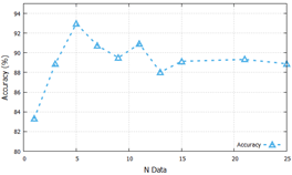
Large sample area sizes and VGG16 architecture were used in this process. The results of this process analysis would be used in the next process. The most optimal result was achieved when the number of samples in the test set was 5. The next process was to evaluate 15 CNN models using the number of sample areas defined in this section.
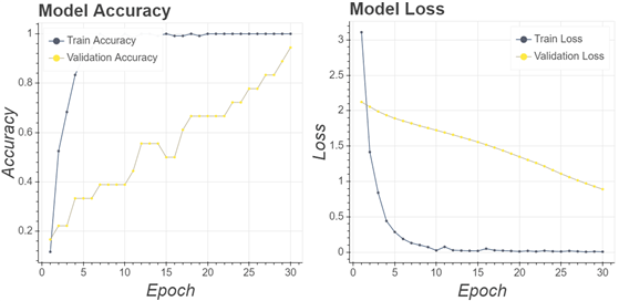
The training process for all CNN models used the same parameters to produce the valid benchmarks. The first training experiment set the following parameters: the number of epochs (30 epochs), learning rate (0.0001), and the optimiser (Adam optimiser). If the training accuracy has not increased in 10 epochs, the training process would be terminated without waiting for the maximum number of epochs. Furthermore, if in 5 epochs training process did not increase, the learning rate would be reduced by multiplying it by a factor value of 0.6. By lowering the learning rate, the process of updating the weight became smoother to increase accuracy. A total of 15 training processes have been completed. Fig. 8 displays a history of training from the VGG16 architecture with a sample size area of 200 pixels.
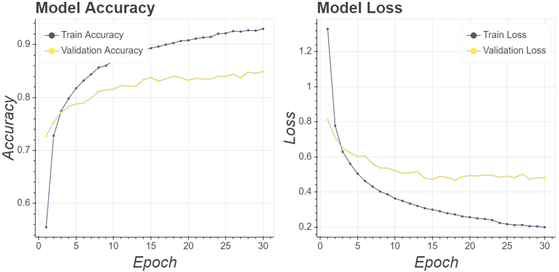
Fig. 8 shows the architecture designed to accept wooden datasets properly. From each epoch, score accuracy continued to increase, and score loss continued to decrease. Scores between the validation and the training were not far apart showing that the model did not overfitting. Furthermore, to test the performance and generalisation of the models, a testing process was carried out on the wood testing dataset that has been prepared.
The testing process was done by evaluating each CNN models with the prepared testing data set. In detailed, the results of the testing process are presented in Table 2.
Based on test results, the accuracy score generally increased following the size of the input image. With a sample area size = 100, the average F1 scores of VGG16, ResNet50, MobileNet, DenseNet121, and Xception were 92, 95, 86, 94, and 92% respectively. With a sample area size = 200, the average F1 scores of VGG16, MobileNet, DenseNet121, and Xception increased to 92, 87, 98, and 96% respectively, and for ResNet50 it decreased to 94%. Finally, for sample area size = 300, the average F1 scores increased for VGG16 and Xception to 94, and 98%, ResNet50 and MobileNet decreased to 89, and 84%, and for DenseNet121 it was unchanged from 98%.
Test result data in Table 2 provides a correlation between the size of the sample area and the capabilities of the resulting CNN model. The size of the sample area is related to the number of features contained in the image. As shown in Fig. 6, the smaller sample area could make the surface features of the wood disappeared due to the cutting process. The samples of medium category area appeared as the most optimal size in maintaining features contained in wood images. This area could create samples containing the most detailed and specific wood features compared to other 2 categories. Proved by the average F1 score of the medium size, each CNN architecture achieved 93.4%. Although the large category sample area had more features, it was not more specific than the medium category sample area. Thus, the results from large area samples did not produce a more general CNN model compared to medium area samples.
Furthermore, Table 2 informs that the DenseNet121- based model became the most general CNN architecture for all sample area sizes and considered to be the best CNN model for Japanese Fagaceae wood identification. DenseNet121-based produced F1 scores above 94% for every size of the sample area (100, 200, and 300 pixels). Meanwhile, MobileNet-based became the CNN architecture providing the lowest accuracy. However, it should be taken into account to use, with the given size of the resulting weight to be the lightest. Although accuracy is not as high as other architectures, it can be the most portable architecture option in use.
To prove how the proposed algorithm could overcome the problems of generalization ability, dataset limitation, and accuracy, several comparisons have been made by making a CNN model that did not go through the sample selection process. In other words, it directly used the original image. As a sample of the training process carried out, Fig. 9 displays the history of the VGG16 architecture training process.
The training process used a similar architecture and parameters as in the training process described in Section 2.4. However, this stage excludes the sample selection process. It resulted in 94% validation accuracy values and validation loss values continuing to approach 0. Implementation of the partial sample area during the training stages does not significantly improve compared to the step with the whole sample area. However, the testing stage obtained different results. As presented in Table 3, most of the CNN architectures provide parameters values at lower levels.
| VGG16 | ResNet50 | MobileNet | DenseNet121 | Xception | |
|---|---|---|---|---|---|
| Precision | 86% | 88% | 51% | 71% | 83% |
| Recall | 81% | 81% | 63% | 67% | 70% |
| F1 | 80% | 81% | 54% | 62% | 70% |
The unfavourable testing results in Table 3 indicated that the model was overfitting and had low generalizability. This comparison showed the advantages and benefits of using the sample selection process. With the similar limited dataset, the sample selection process could overcome the overfitting problem and the low generalizability of the CNN model.
4. CONCLUSION
CNN has become a popular deep learning model widely used for image and visual analysis. In the applications, it requires many datasets to learn a robust classifier. In this wood classification research, the microscopic images taken from the laboratory were in a limited number and had a large size of around 38 Mb and a dimension of 4140 × 3096 pixels. Therefore, a well-designed algorithm has been proposed, which could handle the dataset limitations and identify wood species accurately and efficiently. The proposed algorithm principle was to implement the sample selection process before the dataset entered the classification stage using VGG16, ResNet50, MobileNet, DenseNet121, and Xception based architectures.
The experimental results showed that the sample selection process could produce CNN models with some good generalisation capabilities. The experimental results proved that by making sample areas more specific and detailed, it can produce a powerful CNN model. The medium area sample category (200 × 200 pixels) appeared as the most optimal sample area. While the CNN DenseNet121 architecture became the most optimal architecture when used with medium sample areas.
The availability of more microscopic images is recommended in the future to improve the classification accuracy of the proposed algorithm. The results of this wood classification research are expected to be widely used. With a small size of the CNN model, it can be potentially applied to the mobile devices.
DATA AVAILABILITY STATEMENT
The microscopic images used in the experiment are available from Kyoto University Research Information Repository (https://repository.kulib.kyoto-u.ac.jp/dspace/handle/2433/250016).